How O Make Obi100 Work Again June 2018
1. Introduction
Oracle bone inscriptions (OBI) were recorded from as early on as the Shang Dynasty in Mainland china [1]. The script involves some of the oldest characters in the world and the primeval known form of characters in Communist china and Eastern asia. The characters of OBI have a profound impact on the formation and evolution of Chinese characters, which are usually engraved on animal bones or tortoise shells for the purpose of pyromantic divination [ii,3,4], as shown in Figure one.
Figure 2a shows the characters of OBI corresponding to some normally used words today. We can encounter that characters of OBI were written by drawing shapes and lines based on the shape features of objects, which was one of the most archaic methods of pictographs used by aboriginal people. To engagement, archaeologists have discovered more than than 4500 characters of OBI, but the meanings of half of these characters accept non yet been identified [v]. In the by, experts used manual comparison and analysis to identify the meaning of the characters of OBI based on existing experience, which was effective, only required time and attempt. In addition, since characters of OBI were carved by different groups of ancient people from several historical periods [ii], the characters had big variations in shape, calibration, and orientation. For instance, the eight characters shown in Figure 2b have very like glyphs, but stand for eight words with very different meanings. On the contrary, Figure 2c shows eight characters of OBI written in diverse ways, however, they all express the same meaning of monkey. These pose huge challenges in recognizing characters of OBI.
Recently, some automatic methods for identifying OBI were proposed, among which, feature extraction is the most usually used. Clothes Andreas et al. [6] presented an analysis of oracle bone characters for animals from a cognitive signal of view. Yang [seven] proposed a graph theory to identify OBI, whose core idea was to regard an inscription grapheme as an undirected graph and extract the topological characteristics for recognition. In Li et al.'s work [8], a human being–computer interactive dynamic clarification method was proposed, which described OBI by the stroke–segments–vector and the stroke elements. A Fourier descriptor based on a curvature histogram (FDCH) was proposed by Lu et al. [ix] to represent oracle characters. Gu [x] converted the OBI into topological figures and encoded the topographic figures. Meng [11,12] used the Hough transform to extract line features of characters of OBI, resulting in an inscription recognition accuracy of virtually ninety%. Although feature extraction-based approaches can accomplish the purpose of identifying characters of OBI, they are merely suitable for simple data types or small datasets.
Artificial intelligence (AI) technology has strong potential in OBI recognition, and some researchers applied blueprint recognition and deep learning to the recognition tasks. Support vector motorcar (SVM) [13,14] classification engineering science was used to recognize characters of OBI and reach an accuracy of 88%. Gao et al. [xv] used the Hopfield network for recognizing fuzzy characters of OBI and the highest accuracy rate was 82%. Guo et al. [3] proposed a novel hierarchical representation that combined a Gabor-related low-level representation and a sparse-encoder-related mid-level representation; they combined this method with convolutional neural networks (CNNs) and accomplished 89.1% accuracy in recognition. Although OBI recognition technologies based on deep learning accept adept scalability on big datasets, an overall recognition accuracy withal needs to be improved. In this paper, we explore new approaches to improve the accuracy of OBI recognition using CNNs. Our major contributions are summarized as follows:
-
Nosotros created a dataset named OBI-100 with 100 classes characters of OBI, covering various types of characters, such equally animals, plants, humanity, society, etc., with a total of 4748 samples. Each sample in the dataset was selected carefully from ii definitive dictionaries [16,17]. In view of the diversity of ancient OBI writing styles, we also used rotation, resizing, dilation, erosion, and other transformations to augment the dataset to over 128,000 images. The original dataset can exist found at https://github.com/ShammyFu/OBI-100.git (accessed on 10 Dec 2021).
-
Based on the convolutional neural frameworks of LeNet, AlexNet, and VGGNet, we produced new models by adjusting network parameters and modify network layers. These new models were trained and tested with diverse optimization strategies. From hundreds of different model attempts, 10 CNN models with the all-time performance were selected to identify the 100-grade OBI dataset.
-
The proposed models achieved great recognition results on the OBI dataset, with the highest accuracy charge per unit of 99.5%, which is amend than the three classic network models and better than other methods in the literature.
two. Materials and Methods
2.1. Dataset Preparation
2.1.i. Sample Acquisition
Since characters of OBI are carved on tortoise shells and animal bones, people by and large save them as paper or electronic sample collections by rubbing or taking pictures. The raw data in our dataset come up from two classic scanned OBI dictionaries [xvi,17], both of which are definitive in the field of OBI.
The original dataset contains 100 classes of oracle character samples, of which the smallest category contains twenty samples, and the largest class has 134 examples, with a full of 4748 grapheme images. In social club to ensure the diversity of the dataset, the character categories we select cover humanities, animals, plants, natural environs and activities, etc. Besides, considering that some characters of OBI have many non-standard variants, nosotros select as many of these characters as possible to ensure that the dataset is closer to the reality. This dataset is named OBI-100. Afterward doing this part of the original data collection, we raise the completeness and variety of the dataset through preprocessing, augmentation, and normalization.
2.1.2. Dataset Preprocessing
To restore the writing characteristics of OBI more than accurately, we preprocess the original samples as shown in Figure 3.
-
Denoising: since the OBI samples are from scanned e-books, Gaussian noise was introduced in the images. We first chose the non-local method (NLM) [18] to denoise. For a pixel in an paradigm, this method finds similar regions of that pixel in terms of epitome blocks, and so averages the pixel values in these regions, and replaces the original value of this pixel with the boilerplate value [nineteen], which tin can effectively eliminate Gaussian noise.
-
Binarization: since the OBI images used for recognition crave simply blackness and white pixel values, nosotros converted the denoised samples into grayscale ones and then binarized them.
-
Size normalization: to proceed the size of all images consistent without destroying the useful data areas of them, we rescaled the size of the image to
. For the original non-square images, we filled the blank border area with white pixels first and then scaled them to the required size.
We bear witness examples of the preprocessed dataset in Figure 4.
2.1.3. Data Augmentation
The bereft number of samples in the dataset leads to depression recognition accuracy, so nosotros expand the dataset to amend the effectiveness of the recognition task. Because the randomness of the same character when it is written multiple times, the bending or thickness of the character writing may change. Therefore, we perform several transformations to produce new images, as shown in Figure 5 for each sample.
-
Rotation: generate new images by rotating the original images clockwise or counterclockwise. The rotation angle is randomly selected from 0 to xv degrees.
-
Compress/stretch: adjust the shape of the characters on images by stretching or compressing, using a stretching ratio of 1 to 1.5, and a compression ratio of 0.67 to 1. The deformed images are rescaled to
.
-
Dilation/erosion: dilate or erode the lines of characters of OBI [20] to produce new samples. Due to the small epitome size, directly corrosion will crusade the loss of many features. Nosotros first enlarged the prototype, and then implemented the corrosion operation, and finally resized the image size to
to obtain the all-time corrosion effect.
-
Composite transformation: in addition to the 6 individual transformations described above, we also utilize twenty combinations of transformations to the samples. That is, the image is transformed several times past choosing 2 or more of the above methods to generate the corresponding new samples.
After the augmentation operation, each original image produces 26 corresponding transformed images. The total number of samples increased by 27 times to 128,196 (
). The smallest class contains about 540 images and the largest category has over 3600 images. Information technology presents the number distribution of each category in the OBI dataset in Figure half-dozen.
ii.2. Models Preparation
2.ii.1. Background of CNN
Convolutional neural network (CNN) [21] is a multi-layer feed-forward neural network that can extract features and properties from the input data. Currently, CNN plays an important office in deep learning, considering information technology can learn nonlinear mappings from a very big number of data (images or sounds), even in loftier-dimensional circuitous inputs. In addition, the capability of representation learning enables a CNN to classify input information co-ordinate to its hierarchical construction by translation invariant classification. Specifically, a trained CNN can transform the original image at each layer of the network to produce a grade score corresponding to that input image at the stop of the network [22].
More often than not, equally shown in Effigy 7, the basic CNN structure consists of an input layer, several convolutional layers, and pooling layers, too equally several fully connected layers and an output layer.
The convolutional layer is designed to extract features from the input data, which contain many convolutional kernels. Each element of the kernel corresponds to a weight coefficient and a bias vector. The parameters of the convolutional layer include the size of the kernel, the step size, and the padding method [23]. These three factors jointly determine the size of the output feature map of the convolutional layer [24]. Past introducing an activation function, CNN tin effectively solve various nonlinear problems. The activation function maintains and maps the features of the activated neuron to the next layer. Typically, CNNs utilize the linear rectifier role (rectified linear unit of measurement, ReLU) [25] equally the activation function to help limited circuitous features, which can exist formulated as
. After feature extraction [26] by the convolutional layer, the output feature map is transferred into the pooling layer for feature option and information filtering. The pooling layer actually implements the sampling function, and its main idea is to extract features with a certain trend. For example, max pooling corresponds to more prominent features, while average pooling corresponds to smoother features. The fully connected layer combines the extracted features in a linear style to get the output. The output layer uses a logistic role or a normalized exponential function to output the classification label or probability. Usually, the softmax function [27] is used to calculate the course scores every bit follows:
In the choice of network structure, we trained several mainstream models on the OBI-100 dataset, including LeNet, AlexNet, VGGNet, ResNet-50, and Inception. However, afterwards preliminary experiments, it was found that the results of ResNet-fifty and Inception are not satisfactory (their accuracy rates are both less than 70%). Therefore, we selected 3 network frameworks with stronger performance and college training efficiency: LeNet, AlexNet, and VGGNet. Based on these three models, we adjusted the network structure, modified the parameters, and used various optimization methods to find models with better functioning. After trying hundreds of combinations, we selected x models that performed well. Table 1 summarizes the configuration of these x improved models.
two.2.2. The Improved LeNet Models
LeNet [28] is one of the most representative models for handwritten digit recognition. It consists of two parts: (i) a convolutional encoder consisting of two convolutional layers and two pooling layers; (ii) a dense block consisting of iii fully continued layers. For OBI classification tasks, we propose ii improved models based on LeNet, called L1 and L2. For the two models, we adjusted the original vii-layer construction to a half dozen-layer structure, and adjusted the depth of the convolutional layer and the size of the filter. Specifically, the output dimensions of the convolutional layers and the fully connected layers of the L1 model are basically the same as the original LeNet model, but the 120-depth fully connected layer is direct connected to the concluding 100-depth fully continued layer. On the L2 model, we used a college-dimensional convolution kernel. For example, the beginning convolutional layer uses a 32-dimensional
convolution kernel, and the 2nd convolutional layer uses a 64-dimensional
convolution kernel. In addition, the max pooling method is used in both models. Nosotros prepare the padding parameters of the L1 convolutional layers to the VALID value, which means that the size of the output feature map will change after convolution. Even so, the corresponding parameters of the L2 model are set to SAME, which means that the image size remains unchanged after convolution. Through these aligning strategies, the L1 model inputs 16 characteristic maps with a size of
to the fully connected layer, and L2 inputs 64 feature maps with a size of
.
2.2.3. The Improved AlexNet Models
AlexNet [25] is the winning model in the 2012 ImageNet contest, which consists of 5 convolutional layers, 3 max-pooling layers, two batch normalization layers, ii fully connected layers, and one softmax layer. For AlexNet, we propose three optimized networks to classify characters of OBI, named A1, A2, and A3. These three models have different numbers of convolutional layers and pooling layers, and the commencement 4 convolutional layers take exactly the same structure. Specifically, the A2 model has three more than convolutional layers with 256-dimensional
convolution kernels and a pooling layer than the A1 model. Compared with the A2 model, the A3 model non only improves the depth of the network, just also uses higher-dimensional convolution kernels. In addition, we use the max pooling strategy for all networks. The max pooling layers in the A1 model apply
kernels, while those in the A2 and A3 models use
kernels. In A1 and A3, the pooling layer is added between the last convolutional layer and the fully connected part, whereas the final convolutional layer of the A2 model is directly connected to the first fully continued layer.
two.2.4. The Improved VGGNet Models
Like AlexNet and LeNet, VGGNet [29] can be partitioned into ii parts: the first consisting by and large of convolutional and pooling layers and the second consisting of fully connected layers. The convolutional part of the network connects several VGG blocks in succession and one VGG cake consists of a sequence of convolutional layers, followed by a max pooling layer for spatial downsampling. The concluding of the network is equanimous of three fully connected layers and a softmax layer. Past repeatedly stacking small
kernels and max pooling layers, VGGNet demonstrates remarkable capabilities in feature extraction.
According to the framework of VGGNet, we construct five improved CNNs for OBI character recognition, including V11, V13, V16, V16-2, and V19. The overall construction of these models is adapted from models of dissimilar layers in the VGGNet framework, which are mainly accomplished by calculation or deleting layers in the VGG blocks, adjusting the depth of the convolution kernel, and adjusting the depth of the fully continued layers. For example, comparing with the normal 11-layer structure in VGGNet, 1 convolutional layer is added to each of the first and 2d VGG blocks in V11, while the fourth VGG cake containing 2 convolutional layers in the normal 11-layer structure is deleted in V11.
ii.3. Methods
The recognition experimental method in this section is designed based on the CNN models proposed in Section two.two and the OBI-100 dataset proposed in Department 2.one. In our experiments, the recognition accuracy on the OBI dataset is one of the nigh important indicators for evaluating the operation of these models. Therefore, our target is to train accurate network models. The grooming consequence is related to factors such as the structure of the trained model, the dataset participating in the preparation, the hyperparameter settings and the optimization method used. Thus, nosotros introduce our dataset segmentation approaches, parameter setting strategies and optimization methods used for experiments in the following sections. The models presented in this paper are implemented using TensorFlow, and the paradigm pre-processing process is implemented using OpenCV.
ii.3.one. Dataset Division
The unabridged OBI-100 is divided into a training set, a validation gear up and a test fix at a ratio of approximately eight:one:1. The training set is used to fit the model for prediction or classification. The data from the validation set up assists in the search for optimal hyperparameter combinations, while the examination set is used to evaluate the generalization performance of the selected model. In order to make each category of characters of OBI more uniformly included in each of the to a higher place information subsets, nosotros use the following division process: Firstly, we shuffle the samples of the entire preprocessed OBI-100 dataset fifty times earlier dividing them into different subsets. Secondly, 90% of the images from the sample set are randomly selected and placed in the "train" folder, while the "rest" images are placed in the "examination" binder. We cheque the division results to ensure that each of the 100 classes is included in the to a higher place subsets. Thirdly, the data augmentation methods presented in Section two.1.3 are performed to aggrandize the number of samples in each binder. Fourthly, 10% of the samples in the "train" folder are randomly selected as the validation set, and the rest are used as the final training set. Finally, all data sample files are saved every bit "H5" files for existence loaded during grooming.
2.iii.2. Parameter Setting
The parameter setting mainly includes two aspects, 1 is the weight initialization strategy of the network, and the other is the hyperparameter configuration scheme for model training. Choosing a suitable initial configuration has a crucial touch on the unabridged grooming process. For example, reasonable hyperparameters can prevent the network from entering a certain layer of forrad (or astern) saturation prematurely. The weight initialization methods commonly include zero initialization, random initialization, and He initialization [30]. After many experiments, we empirically adopt He Initialization and set the initial bias to 0.one. In terms of training hyperparameters, the preparation epoch of all our networks is set to 100, and the discrete staircase method is used for model grooming, where the learning rate is initially set to 0.1 and halved every 20 epochs. Moreover, we ready the batch size of the training dataset to the value in (32, 64, 96, 128, 160, 196, 224, 256). Nosotros used different parameter combinations to conduct experiments and observed the training process and effects of these models, and then we selected the optimal parameter configuration schemes.
2.3.iii. Optimization Methods
In addition to setting a set of appropriate grooming parameters, in order to further ameliorate the training issue of the network, we also applied some optimization methods.
-
Batch normalization [31]: batch normalization normalizes the input of each small batch to i layer, which has the result of stabilizing the learning process and can significantly reduce the training time required for training deep networks. In our experiment, when using this optimization method, the batch normalization layer is added before each activation function to make the distribution of the data render to the normalized distribution, and so that the input value of the activation function falls in the region where the activation function is more sensitive to the input.
-
Dropout [32]: by randomly removing the nodes of the network during the training process, a unmarried model can simulate a large number of different architectures, which is called the dropout method. Information technology provides a very low computational toll and very constructive regularization approach to alleviate overfitting of deep neural networks and better the generalization performance. When this method is used in our experiments, nosotros add together a dropout layer to each fully connected layer, which reduces the interdependence betwixt the neuron nodes in the network by deactivating some neurons with a certain probability value (making the output of the neurons zero). In our experiment, we railroad train models by jointly adjusting the probability value of the dropout layer and the batch size value. First, nosotros try to set the probability value of dropout layers to the value in (0.i, 0.2, 0.3, 0.four, 0.5, 0.6, 0.7, 0.eight, 0.9, i). Second, through multiple experiments, we select the best combination of dropout and batch size values.
-
Shuffle: to eliminate the potential impact of the order in which the training information are fed into the network and farther increase the randomness of the training data samples, we introduce the shuffle method into the model evaluation experiments. Specifically, when this method is applied, we shuffle all training samples in each new preparation epoch, and then input each shuffled information batch into the network.
iii. Results
To notice models with stable performance and high OBI grapheme recognition accuracy among the ten proposed CNN models, we conducted the following three kinds of experiments and observed each set of experimental results.
-
We visualized the changes in the preparation loss value, the accurateness rates on the training set and the validation set of unlike models during the training process as the number of preparation epochs increases. In add-on, past comparing the training accurateness and validation accuracy, we can infer the overall learning effect of the models respective to each epoch. These are discussed in Department three.one.
-
For different models, we test the bear on of multiple combinations of batch size value and dropout probability value on recognition accuracy of the validation set. By comparison, the optimal combination of these two parameters is selected as the setting strategy for the final performance experiment of the corresponding model. The results are mainly analyzed in Department three.2.
-
From the three aspects of data augmentation, model structure adjustment, and optimization implementation, we evaluate the furnishings of various improvement methods on model learning and OBI recognition. Results and discussions are presented in Section three.three.
3.1. Grooming Process Observation
For the three groups of improved models corresponding to the three basic CNN frameworks, we chose one from each grouping to observe the corresponding preparation process, every bit shown in Figure 8, Figure 9 and Figure 10. For each left graph, the bluish line represents the validation accuracy (recognition accurateness on the validation gear up), and the carmine line refers to the training accurateness (recognition accuracy on the grooming set). Each figure on the correct shows the relationship between training loss and training epochs.
The training process of the L2 model (ane of the improved LeNet models) is shown in Figure viii. We can see that, in the first ten epochs of grooming, the training loss value drops sharply and the training accurateness rises dramatically, indicating that the model is learning effectively. From the 10th epoch to the 40th epoch, the training loss still shows a downwardly trend until it stabilizes subsequently 40 epochs, which is also consistent with the alter in training accuracy. Nevertheless, although the validation accuracy charge per unit is too on the ascent, when budgeted 100 epochs, the training set accuracy rate is close to 1, while the accuracy rate on the validation set is lower than 90% and continues to fluctuate, which demonstrates that only training for 100 epochs cannot make the L2 model fully converge.
For the A3 model (ane of the improved AlexNet models) in Effigy 9, the accuracy rates on the preparation set and the validation set basically maintain a consistent trend on the whole. Specifically, in the get-go x epochs of training, both curves ascent speedily. Afterwards 10 epochs, the training accuracy gradually tends to 100% and becomes smoothen, while the validation accuracy curve still has large fluctuations. This suggests that the learning of the A3 model is not stable plenty despite the high recognition accuracy within 100 epochs.
The grooming procedure of the V16 model (i of the improved VGGNet models) is shown in Figure 10. From these two graphs, we can conspicuously detect that on the V16 model, both the training and validation accuracy rates increment with very sharp fluctuations in the first 40 epochs, and these fluctuations also occur on the training loss curve. However, after the 40th epoch, the preparation and validation accuracy curves are smoothed effectually 100%, and the training accuracy is slightly college than the validation accuracy. From this nosotros conclude that the V16 model merely needs about twoscore epochs to converge and has expert recognition functioning.
3.2. Parameter Upshot Evaluation
We keep the other hyperparameters of the network unchanged and accommodate the values of batch size and dropout probability associatively to observe the recognition accuracy on the validation gear up of the model, where the value of batch size is taken from (32, 64, 96, 128, 160, 192, 224, 256) and that of dropout probability is taken from (0.1, 0.2, 0.3, 0.4, 0.5, 0.half dozen, 0.7, 0.8, 0.9, ane). Surface plots of the relationship between batch size, dropout probability and validation accuracy rate on L2, A3 and V16 models are obtained as Figure 11, Effigy 12 and Figure 13, respectively. We use a black dot to marker the point with the highest accuracy on each surface, and mark the respective 10 and y coordinates side by side to that point.
According to the colour change of the surface plots, it tin be inferred that the more desperate the color system changes, the greater the impact of dissimilar choices of values of the batch size and the dropout probability on the models is. From Effigy 11 nosotros see that at that place are obvious bluish and yellow areas, indicating that the accuracy of the L2 model is most affected past these two parameters, followed by the A3 model in Effigy 12. The color system of the surface map in Figure 13 corresponding to the V16 model changes smoothly, so it is minimally affected by the two parameters. In add-on, the highest point indicates the optimal combination of batch size and dropout probability values. For the L2 and A3 models, setting the batch size and dropout probability values to 64 and 0.v is the optimal choice, while for the V16 model, they should be set to 128 and 0.six, respectively.
3.3. Model Performance Overview
From the above experimental results, we obtain the best combination of batch size and dropout probability values used to train each model. In the next experiment, we use the optimization methods mentioned in Section 2.iii.three and the optimal hyperparameter combination configurations to train the classical and the proposed improved models. In improver, to evaluate the issue of data augmentation for the OBI-100 dataset, these models are also trained and tested on the not-augmented dataset. A full general overview of the final results is shown in Table 2, Table 3 and Table four.
From Table 2, Table 3 and Table iv, on the ane manus, nosotros can but observe that the data augmentation strategy tin generally enhance the recognition accuracy of the models. For instance, the L1 model trained on the shuffled unaugmented training set up gets a maximum accuracy of only 78.77% for the simpler unaugmented test set nomenclature chore, while the L1 model learned on the augmented OBI-100 yields an accuracy of 95.35% against the more than difficult augmented sample recognition job. On the other hand, nosotros observe that compared with the original models of the three classic frameworks, the improved networks show amend recognition functioning on the augmented OBI dataset. Specifically, when integrating the three optimization methods, the L1 and L2 models achieve xiii.02% and 11.47% higher recognition performance than the original LeNet respectively, while the A1, A2, and A3 models yield 5.09%, 5.39%, and 6.82% improvement in recognition accuracy respectively, compared to the original AlexNet. In add-on, the performance baseline of the original VGGNet-based models is relatively loftier, just the improved model even so results in functioning gains. For case, the accuracy of the optimal V16 model is 99.fifty%, while the original VGG16 model only achieves 97.75%.
Moreover, adding suitable optimization methods contributes a lot to the recognition accurateness of the models. For instance, for the V11 model trained on the augmented OBI-100, the maximum exam accuracy reaches 91.twenty% when using batch normalization only, and the accurateness is enhanced to 91.80% after using shuffle optimization, and it is further improved to 94.66% after applying the dropout method. Similar accuracy improvements tin be clearly observed in the experimental results of each proposed model.
For each group of enhanced models, we also make the post-obit observations. Firstly, the LeNet-based L1 model is significantly better than the L2 model. On the i hand, the best maximum exam accuracy of the L1 model is higher than that of the L2 model, and on the other hand, the gap between the maximum test rate and the average test rate of the L1 model is a smaller value of 0.five%, indicating that the training result of the L1 model is more stable.
Thirdly, from Tabular array iv, one can see that the increase in the number of network layers has a beneficial effect on the recognition performance of the VGGNet-based models. Specifically, V11, V13, and V16 with the same fully continued layer structures, respectively, get the best accurateness rates of 94.66%, 95.85%, and 99.50%, incrementally. In addition, for V16 and V16-two with the same network structures of convolutional and pooling layers, the V16 model with deeper fully continued layers outperforms the V16-2 model by iii.9%. Nosotros likewise detect that the maximum accuracy on the V16 model is the same equally the average accuracy, indicating that the V16 model performs more than effective feature learning on the OBI-100 dataset.
Finally, from Table 2, Table iii and Table 4, information technology is obtained that the VGGNet-based V16 model, for one, achieves the highest accurateness of 99.v% on the OBI-100 dataset, for another, the maximum and boilerplate accuracy values of this model are the same, and so it is the all-time model for identifying the OBI-100 dataset in our experiments.
4. Conclusions
In this piece of work, deep convolutional neural networks are used to identify oracle characters. We created a standardized dataset called OBI-100, which contains 100 classes of characters of OBI. OBI-100 tin fill the gap of publicly available datasets in the applications of deep learning in OBI research. Base on three typical convolutional network frameworks, ten improved models are proposed to classify the characters of OBI. Through a large number of experiments and a diversity of optimization methods, the all-time model achieves an accuracy of 99.5% in the 100-class OBI recognition task. Our piece of work shows that characters of OBI can exist recognized practically and effectively in deep convolutional neural networks, and applications in this area take broad research prospects, which too provide new ideas for studying the origin of words and human history.
Author Contributions
Conceptualization, Xuanming Fu and Zhengfeng Yang; methodology, Xuanming Fu, Zhengfeng Yang, and Zhenbing Zeng; software, Yidan Zhang and Qianting Zhou; validation, Yidan Zhang and Qianting Zhou; formal analysis, Xuanming Fu and Zhengfeng Yang; investigation, Yidan Zhang; resources, Qianting Zhou; data curation, Xuanming Fu and Qianting Zhou; writing—original draft grooming, Xuanming Fu; writing—review and editing, Xuanming Fu, Zhengfeng Yang and Zhenbing Zeng; visualization, Yidan Zhang and Qianting Zhou; supervision, Zhengfeng Yang and Zhenbing Zeng; project administration, Qianting Zhou. All authors have read and agreed to the published version of the manuscript.
Funding
This research was supported by Henan Cardinal Laboratory of Oracle Bone Inscription Information Processing (AnYang Normal Academy), grant number 2021ZR0101.
Institutional Review Board Statement
Not applicable.
Informed Consent Argument
Non applicative.
Data Availability Statement
Conflicts of Interest
The authors declare no conflict of involvement.
References
- Keightley, D.Due north. The Shang State as Seen in the Oracle-Bone Inscriptions. Early China 1980, v, 25–34. [Google Scholar] [CrossRef]
- Flad, R.Thou. Divination and Power: A Multiregional View of the Development of Oracle Bone Divination in Early China. Curr. Anthropol. 2008, 49, 403–437. [Google Scholar] [CrossRef]
- Guo, J.; Wang, C.; Rangel, E.R.; Chao, H.; Rui, Y. Building Hierarchical Representations for Oracle Graphic symbol and Sketch Recognition. IEEE Trans. Epitome Process. 2015, 25, 104–118. [Google Scholar] [CrossRef] [PubMed]
- Keightley, D.N. Graphs, Words, and Meanings: Three Reference Works for Shang Oracle-Bone Studies, with an Excursus on the Religious Function of the Day or Sun. J. Am. Orient. Soc. 1997, 117, 507–524. [Google Scholar] [CrossRef]
- Bazerman, C. Handbook of research on writing: History, order, school, individual, text. Delta Doc. Estud. Lingüística Teórica E Apl. 2008, 24, 419–420. [Google Scholar]
- Dress, A.; Grünewald, Due south.; Zeng, Z. A cerebral network for oracle bone characters related to animals. Int. J. Modernistic. Phys. B 2016, 30, 1630001. [Google Scholar] [CrossRef]
- Feng, Y. Recognition of jia gu wen based on graph theory. J. Electron. Inf. Technol. 1996, 18, 41–47. [Google Scholar]
- Li, Q.; Wu, Q.; Yang, Y. Dynamic Clarification Library for Jiaguwen Characters and the Reserch of the Characters Processing. Acta Sci. Nat. Univ. Pekin. 2013, 49, 61–67. [Google Scholar]
- Lu, 10.; Li, M.; Cai, K.; Wang, 10.; Tang, Y. A graphic-based method for Chinese Oracle-bone classification. J. Beijing Inf. Sci. Technol. Univ. 2010, 25, 92–96. [Google Scholar]
- Gu, S. Identification of Oracle-bone Script Fonts Based on Topological Registration. Comput. Digit. Eng. 2016, 44, 2001–2006. [Google Scholar]
- Meng, L. 2-Phase Recognition for Oracle Os Inscriptions. In Proceedings of the ICIAP, Catania, Italy, 11–15 September 2017. [Google Scholar]
- Meng, L. Recognition of Oracle Bone Inscriptions by Extracting Line Features on Paradigm Processing. In Proceedings of the ICPRAM, Porto, Portugal, 24–26 Feb 2017. [Google Scholar]
- Liu, Y.; Liu, 1000. Oracle grapheme recognition based on SVM. J. Anyang Norm. Univ. 2017, 2, 54–56. [Google Scholar]
- Gjorgjevikj, D.; Cakmakov, D. Handwritten Digit Recognition by Combining SVM Classifiers. In Proceedings of the Eurocon 2005—The International Conference on "reckoner equally a Tool", Belgrade, Serbia, 21–24 November 2005. [Google Scholar]
- Gao, F.; Xiong, J.; Liu, Y. Recognition of Fuzzy Characters on Oracle-Bone Inscriptions. In Proceedings of the IEEE International Conference on Figurer & It; Ubiquitous Computing & Communications; Undecayed, Autonomic and Secure Computing; Pervasive Intelligence and Computing, Liverpool, UK, 26–28 October 2015. [Google Scholar]
- Institute of Archæology, Chinese Academy of Sciences. Oracle Bone Inscriptions Collection; Zhonghua Book Company: Beijing, Cathay, 1965. [Google Scholar]
- Wang, B. 100 Cases of Classical Oracle Bone Inscription Rubbings; Beijing Arts and crafts Publishing House: Beijing, China, 2015. [Google Scholar]
- Froment, J. Parameter-Costless Fast Pixelwise Not-Local Means Denoising. Image Process. Line 2014, iv, 300–326. [Google Scholar] [CrossRef]
- Buades, A.; Coll, B.; Morel, J.M. Non-Local Ways Denoising. Image Process. Line 2011, one, 208–212. [Google Scholar] [CrossRef]
- Chen, S.; Haralick, R.M. Recursive Erosion, Dilation, Opening, and Closing Transforms. IEEE Trans. Paradigm Procedure. 1995, 4, 335–345. [Google Scholar] [CrossRef] [PubMed]
- Kim, P. Convolutional Neural Network In MATLAB Deep Learning: With Car Learning, Neural Networks and Artificial Intelligence; Apress: Berkeley, CA, USA, 2017. [Google Scholar]
- Maitra, D.S.; Bhattacharya, U.; Parui, S.K. CNN based mutual arroyo to handwritten character recognition of multiple scripts. In Proceedings of the 2015 13th International Briefing on Certificate Analysis and Recognition (ICDAR), Tunis, Tunisia, 23–26 August 2015. [Google Scholar]
- Heaton, J. Deep learning. Genet. Program. Evolvable Mach. 2018, 19, 305–307. [Google Scholar] [CrossRef]
- Hinton, G.E.; Osindero, Southward.; Teh, Y.W. A Fast Learning Algorithm for Deep Belief Nets. Neural Comput. 2006, 18, 1527–1554. [Google Scholar] [CrossRef] [PubMed]
- Krizhevsky, A.; Sutskever, I.; Hinton, G.E. ImageNet Classification with Deep Convolutional Neural Networks. In Proceedings of the International Conference on Neural Information Processing Systems, Lake Tahoe, NV, United states, 3–6 December 2012. [Google Scholar]
- Zhou, B.; Lapedriza, A.; Xiao, J.; Torralba, A.; Oliva, A. Learning Deep Features for Scene Recognition using Places Database. Adv. Neural Inf. Process. Syst. 2015, one, 487–495. [Google Scholar]
- Bishop, C.M. Neural Networks for Blueprint Recognition. Agric. Eng. Int. Cigr J. Sci. Res. Dev. Manuscr. Pm 1995, 12, 1235–1242. [Google Scholar]
- Le Cun, Y.; Jackel, L.D.; Boser, B.; Denker, J.S.; Graf, H.P.; Guyon, I.; Henderson, D.; Howard, R.East.; Hubbard, W. Handwritten Digit Recognition: Applications of Neural Net Chips and Automatic Learning. IEEE Commun. Mag. 1989, 27, 41–46. [Google Scholar] [CrossRef]
- Simonyan, Thousand.; Zisserman, A. VVery Deep Convolutional Networks for Large-Calibration Image Recognition. In Proceedings of the 3rd International Conference on Learning Representations, ICLR 2015, San Diego, CA, United states of america, 7–9 May 2015. [Google Scholar]
- He, K.; Zhang, 10.; Ren, S.; Sun, J. Delving Deep into Rectifiers: Surpassing Homo-Level Functioning on ImageNet Classification. In Proceedings of the ICCV, Santiago, Republic of chile, seven–13 December 2015. [Google Scholar]
- Ioffe, Southward.; Szegedy, C. Batch normalization: Accelerating deep network grooming by reducing internal covariate shift. In Proceedings of the International Conference on Machine Learning, Lille, French republic, 7–9 July 2015. [Google Scholar]
- Srivastava, N.; Hinton, G.; Krizhevsky, A.; Sutskever, I.; Salakhutdinov, R. Dropout: A Elementary Manner to Preclude Neural Networks from Overfitting. J. Mach. Learn. Res. 2014, xv, 1929–1958. [Google Scholar]
Effigy ane. The abdominal parts of 2 tortoise shells with divinatory inscriptions excavated at the site of Yinxu, Anyang, Henan, China.
Effigy one. The abdominal parts of ii tortoise shells with divinatory inscriptions excavated at the site of Yinxu, Anyang, Henan, China.
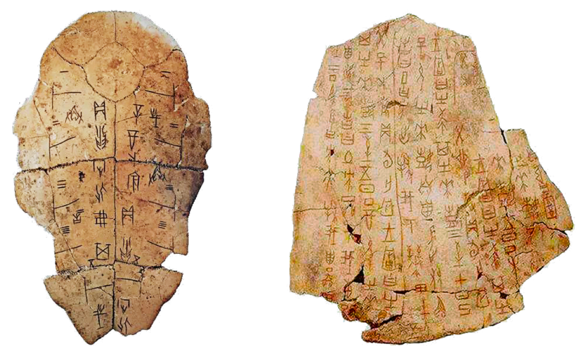
Figure 2. Examples of OBI characters. (a) Examples of characters of OBI corresponding to viii commonly used words. (b) Viii characters of OBI that have different meanings, only look very similar. (c) Eight writing styles of monkey in OBI.
Effigy 2. Examples of OBI characters. (a) Examples of characters of OBI corresponding to eight usually used words. (b) 8 characters of OBI that accept different meanings, merely look very similar. (c) Eight writing styles of monkey in OBI.
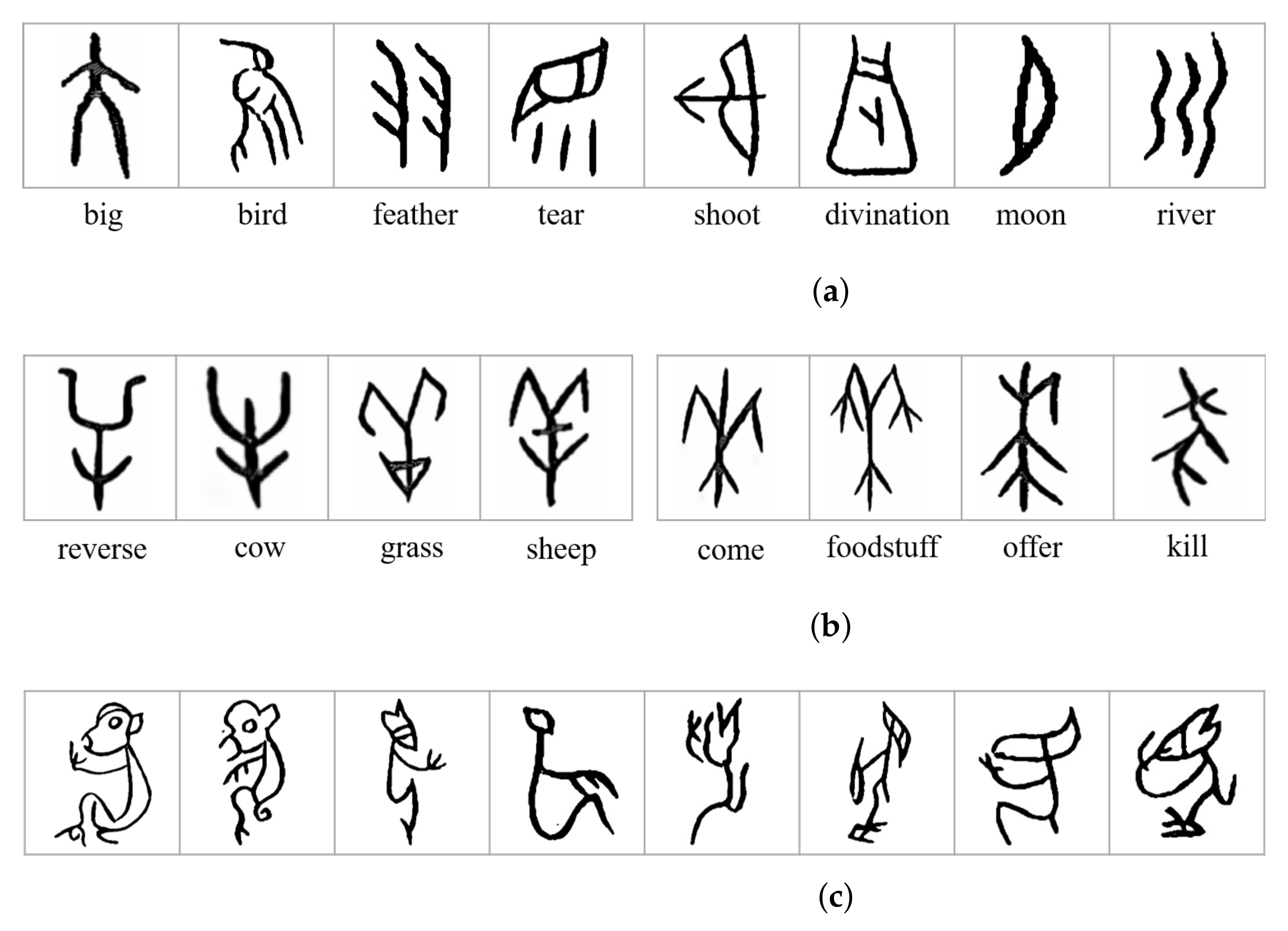
Figure 3. The preprocessing process of OBI character "monkey".
Effigy 3. The preprocessing process of OBI character "monkey".
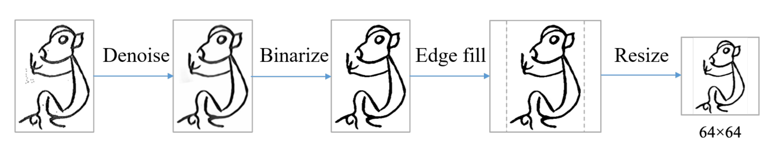
Figure 4. Examples of OBI-100 dataset.
Figure 4. Examples of OBI-100 dataset.
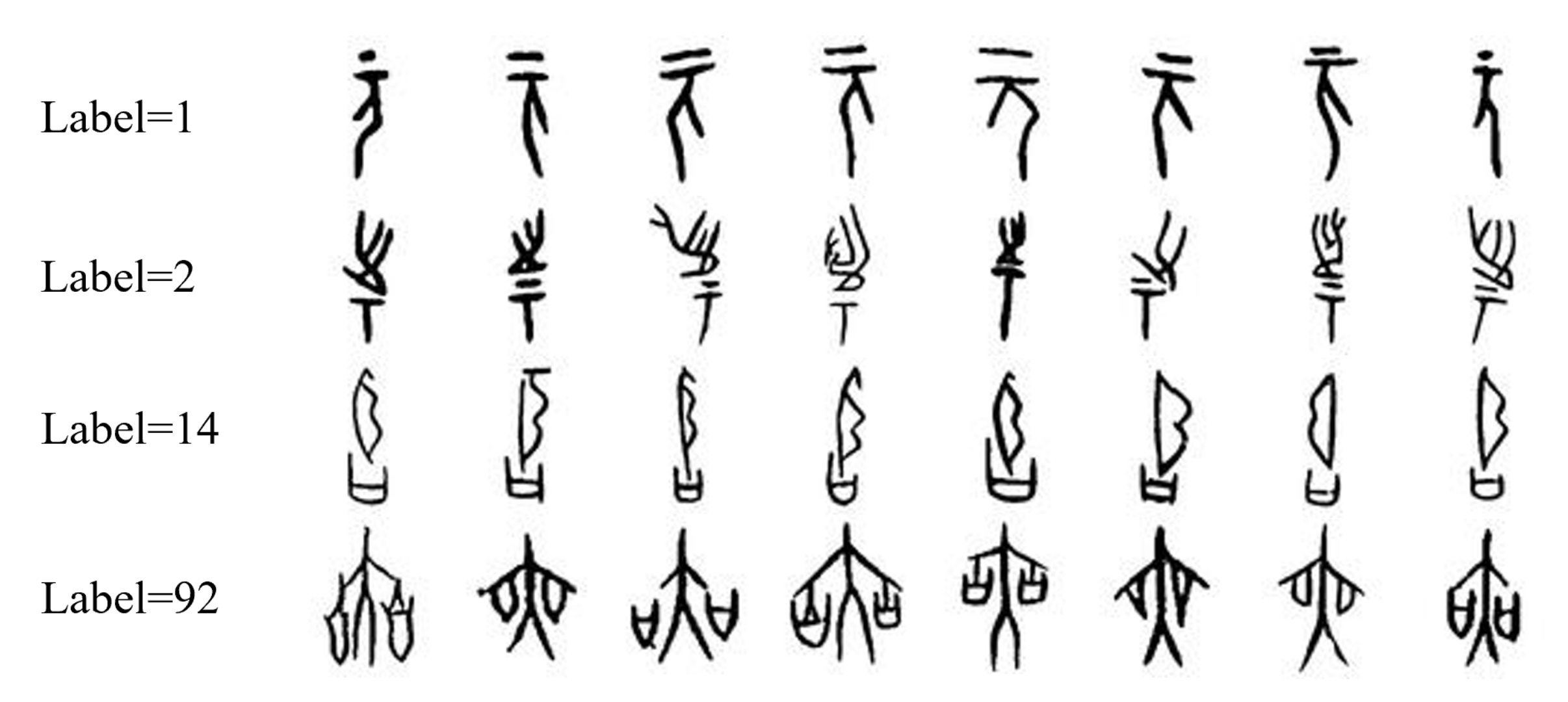
Figure 5. An example of data augmentation.
Figure five. An instance of data augmentation.
Figure 6. The number of samples in each category of the augmented OBI-100 dataset.
Effigy 6. The number of samples in each category of the augmented OBI-100 dataset.

Figure 7. The basic structure of CNN.
Effigy vii. The basic structure of CNN.

Effigy eight. Training accurateness, validation accuracy, and grooming loss during L2 model training. (a) Accuracy comparing. (b) Cross loss.
Figure 8. Training accuracy, validation accuracy, and training loss during L2 model preparation. (a) Accuracy comparison. (b) Cross loss.
Figure 9. Preparation accuracy, validation accurateness and training loss during A3 model preparation. (a) Accurateness comparing. (b) Cross loss.
Figure ix. Training accurateness, validation accuracy and preparation loss during A3 model preparation. (a) Accuracy comparing. (b) Cross loss.
Figure 10. Training accurateness, validation accurateness, and training loss during V16 model training. (a) Accuracy comparison. (b) Cross loss.
Figure 10. Preparation accurateness, validation accuracy, and training loss during V16 model training. (a) Accuracy comparison. (b) Cantankerous loss.

Figure 11. Surface plot on the L2 model displaying the resulting validation recognition accuracy for unlike choices of values of the batch size and the dropout probability.
Effigy xi. Surface plot on the L2 model displaying the resulting validation recognition accuracy for different choices of values of the batch size and the dropout probability.
Figure 12. Surface plot on the A3 model displaying the resulting validation recognition accurateness for dissimilar choices of values of the batch size and the dropout probability.
Figure 12. Surface plot on the A3 model displaying the resulting validation recognition accuracy for different choices of values of the batch size and the dropout probability.

Figure 13. Surface plot on the V16 model displaying the resulting validation recognition accurateness for different choices of values of the batch size and the dropout probability.
Figure 13. Surface plot on the V16 model displaying the resulting validation recognition accurateness for different choices of values of the batch size and the dropout probability.
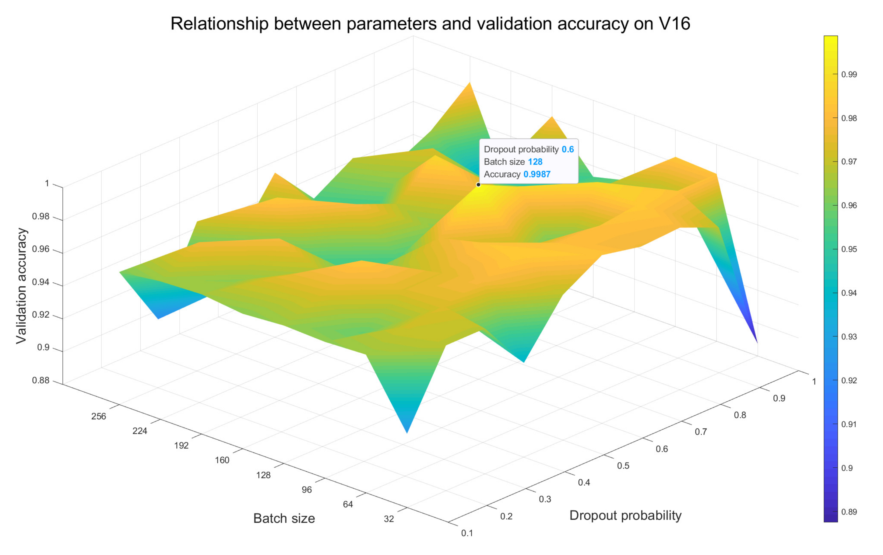
Table ane. Convolutional neural network configurations. Input: greyness-scale images with a size of
from OBI-100. Conv x-y: a convolutional layer with a kernel size of
and an output dimension of the feature map of y. FC-y: a fully connected layer with an output dimension of the feature map of y; maxpool: : a max pooling layer with a kernel size of
. All network models utilize ReLU as the activation function and utilize softmax to summate cantankerous entropy loss.
Table 1. Convolutional neural network configurations. Input: grey-scale images with a size of
from OBI-100. Conv x-y: a convolutional layer with a kernel size of
and an output dimension of the characteristic map of y. FC-y: a fully continued layer with an output dimension of the feature map of y; maxpool: : a max pooling layer with a kernel size of
. All network models use ReLU equally the activation function and utilize softmax to calculate cross entropy loss.
| ConvNet Configurations | ||||||||||
|---|---|---|---|---|---|---|---|---|---|---|
| Framework | LeNet | AlexNet | VGGNet | |||||||
| Name of our proposed Models | L1 | L2 | A1 | A2 | A3 | V11 | V13 | V16 | V16-2 | V19 |
| Input | gray-scale images from OBI-100. | |||||||||
| Network Structure | conv5-6 | conv3-32 | conv11-64 | conv11-64 | conv11-64 | conv3-64 conv3-64 | conv3-32 conv3-32 | conv3-64 conv3-64 | conv3-64 conv3-64 | conv3-64 conv3-64 conv3-64 |
| maxpool: | maxpool: | maxpool: | maxpool: | |||||||
| conv5-16 | conv5-64 | conv5-192 | conv5-192 | conv5-192 | conv3-128 conv3-128 | conv3-64 conv3-64 | conv3-64 conv3-64 | conv3-64 conv3-64 | conv3-128 conv3-128 conv3-128 | |
| maxpool: | maxpool: | maxpool: | maxpool: | |||||||
| conv3-384 conv3-256 | conv3-384 conv3-256 conv3-256 | conv3-384 conv3-256 conv3-256 | conv3-256 conv3-256 | conv3-128 conv3-128 | conv3-128 conv3-128 conv3-128 | conv3-128 conv3-128 conv1-128 | conv3-256 conv3-256 conv3-256 | |||
| maxpool: | maxpool: | maxpool: | ||||||||
| conv3-256 conv3-256 | conv3-512 conv3-1024 conv3-1024 | conv3-512 conv3-512 | conv3-256 conv3-256 | conv3-256 conv3-256 conv3-256 | conv3-256 conv3-256 conv1-256 | conv3-512 conv3-512 conv3-512 | ||||
| maxpool: | maxpool: | |||||||||
| conv3-512 conv3-512 | conv3-512 conv3-512 conv3-512 | conv3-512 conv3-512 conv1-512 | conv3-512 conv3-512 conv3-512 conv3-512 | |||||||
| maxpool: | ||||||||||
| FC-120 | FC-512 | FC-4096 FC-4096 | FC-1024 FC-1024 | FC-4096 FC-4096 | FC-4096 FC-4096 | FC-4096 FC-4096 | FC-4096 FC-4096 | FC-1024 FC-1024 | FC-4096 FC-4096 | |
| FC-100 | ||||||||||
| softmax | ||||||||||
Table 2. Recognition accuracy of LeNet-based models on unaugmented (No) and augmented (Yes) OBI datasets. BN, DP, SF stand for batch normalization, dropout, and shuffle methods, respectively. Examination (max) denotes the maximum recognition accuracy charge per unit and Test (ave) represents the boilerplate value of the concluding five accurateness rates subsequently the grooming is stable. Bold numbers signal the optimal value of each indicator in each group of network frameworks.
Table two. Recognition accuracy of LeNet-based models on unaugmented (No) and augmented (Yeah) OBI datasets. BN, DP, SF correspond batch normalization, dropout, and shuffle methods, respectively. Test (max) denotes the maximum recognition accurateness rate and Test (ave) represents the average value of the last v accurateness rates after the training is stable. Assuming numbers indicate the optimal value of each indicator in each group of network frameworks.
| Model | Data Augment | Method | Accuracy (%) | |
|---|---|---|---|---|
| Test (Max) | Test (Ave) | |||
| Based on LeNet | ||||
| LeNet | No | - | 71.23 | - |
| L1 | SF | 78.77 | 78.77 | |
| L2 | SF | 74.20 | - | |
| LeNet | Yes | - | 81.25 | 75.00 |
| SF + BN + DP | 85.41 | 82.37 | ||
| L1 | SF | 95.35 | 92.48 | |
| SF + BN | 97.15 | 96.56 | ||
| SF + BN + DP | 98.43 | 97.93 | ||
| L2 | SF | 93.75 | 87.fifty | |
| SF + BN | 94.25 | 88.80 | ||
| SF + BN + DP | 96.88 | 86.93 | ||
Table 3. Recognition accuracy of AlexNet-based models on unaugmented (No) and augmented (Yeah) OBI datasets. BN, DP, SF stand for batch normalization, dropout, and shuffle methods, respectively. Test (max) denotes the maximum recognition accuracy rate and Test (ave) represents the boilerplate value of the last 5 accuracy rates afterward the training is stable. Bold numbers point the optimal value of each indicator in each group of network frameworks.
Table 3. Recognition accuracy of AlexNet-based models on unaugmented (No) and augmented (Yes) OBI datasets. BN, DP, SF represent batch normalization, dropout, and shuffle methods, respectively. Test (max) denotes the maximum recognition accurateness rate and Test (ave) represents the average value of the last five accuracy rates subsequently the training is stable. Bold numbers indicate the optimal value of each indicator in each group of network frameworks.
| Model | Data Broaden | Method | Accuracy (%) | |
|---|---|---|---|---|
| Exam (Max) | Test (Ave) | |||
| Based on AlexNet | ||||
| AlexNet | No | - | 71.23 | - |
| A1 | DP | 84.47 | - | |
| A2 | DP + SF | 89.80 | - | |
| A3 | DP + SF | 91.32 | - | |
| AlexNet | Yes | - | 79.40 | 76.91 |
| DP + SF + BN | 91.66 | 89.97 | ||
| A1 | DP | 92.19 | 92.17 | |
| DP + SF | 94.12 | 93.xi | ||
| DP + SF + BN | 96.75 | 94.05 | ||
| A2 | DP + SF | 96.88 | 91.04 | |
| DP + SF + BN | 97.05 | 93.76 | ||
| A3 | DP + SF | 98.44 | 93.25 | |
| DP + SF + BN | 98.48 | 95.38 | ||
Table 4. Recognition accuracy of VGGNet-based models on unaugmented (No) and augmented (Yes) OBI datasets. VGG due north refers to the standard VGGNet model with a n-layer structure. BN, DP, SF correspond batch normalization, dropout, and shuffle methods, respectively. Test (max) denotes the maximum recognition accuracy rate and test (ave) represents the boilerplate value of the concluding five accuracy rates after the preparation is stable. Bold numbers indicate the optimal value of each indicator in each grouping of network frameworks.
Table iv. Recognition accuracy of VGGNet-based models on unaugmented (No) and augmented (Aye) OBI datasets. VGG n refers to the standard VGGNet model with a north-layer structure. BN, DP, SF stand for batch normalization, dropout, and shuffle methods, respectively. Test (max) denotes the maximum recognition accuracy charge per unit and test (ave) represents the average value of the last five accurateness rates after the training is stable. Bold numbers indicate the optimal value of each indicator in each grouping of network frameworks.
| Model | Information Broaden | Method | Accuracy (%) | |
|---|---|---|---|---|
| Exam (Max) | Test (Ave) | |||
| Based on VGGNet | ||||
| VGG11 | No | - | 84.88 | - |
| V11 | BN | 85.56 | - | |
| VGG13 | - | 85.03 | - | |
| V13 | BN + SF | 85.10 | - | |
| VGG16 | - | 93.75 | - | |
| V16 | BN + SF | 91.28 | - | |
| VGG19 | - | 90.35 | - | |
| V19 | BN + SF | 89.71 | - | |
| Based on VGGNet | ||||
| VGG11 | Yeah | - | 91.10 | 90.39 |
| BN + SF + DP | 92.96 | 92.eighteen | ||
| V11 | BN | 91.twenty | 91.10 | |
| BN + SF | 91.fourscore | 91.20 | ||
| BN + SF + DP | 94.66 | 92.fifty | ||
| VGG13 | - | 92.88 | xc.67 | |
| BN + SF + DP | 94.31 | 93.21 | ||
| V13 | BN + SF | 93.20 | 91.75 | |
| BN + SF + DP | 95.85 | 95.10 | ||
| VGG16 | - | 96.24 | 93.75 | |
| BN + SF + DP | 97.75 | 95.65 | ||
| V16 | BN + SF | 99.49 | 99.00 | |
| BN + SF + DP | 99.fifty | 99.50 | ||
| V16-2 | BN + SF | 95.30 | 94.thirteen | |
| BN + SF + DP | 95.60 | 94.38 | ||
| VGG19 | - | 96.67 | 96.28 | |
| BN + SF + DP | 98.26 | 97.75 | ||
| V19 | BN + SF | 98.40 | 98.xx | |
| BN + SF + DP | 98.75 | 98.61 | ||
| Publisher's Note: MDPI stays neutral with regard to jurisdictional claims in published maps and institutional affiliations. |
© 2022 past the authors. Licensee MDPI, Basel, Switzerland. This article is an open up access commodity distributed under the terms and weather of the Creative Commons Attribution (CC By) license (https://creativecommons.org/licenses/by/iv.0/).
killeenthatter1999.blogspot.com
Source: https://www.mdpi.com/2220-9964/11/1/45/htm
Post a Comment for "How O Make Obi100 Work Again June 2018"